E-Learning Portal

Introduction

Microsoft Excel is a helpful and powerful program for data analysis and documentation. It is a spreadsheet program, which contains a number of columns and rows, where each intersection of a column and a row is a “cell.” Each cell contains one point of data or one piece of information. By organizing the information in this way, you can make information easier to find, and automatically draw information from changing data.

Basics

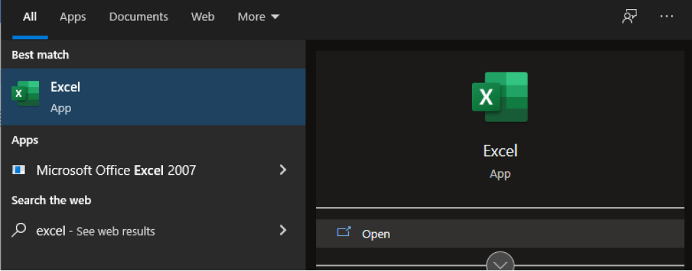
Open MS-Excel

Step 1:

Click on search icon

Step 2:

Type Excel

Step 3:

Click on Open and wait for it to Start

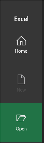
Open an existing Excel Sheet:

Step 1:

Click Open from the File tab

Step 2:

Select Browse under Open Section

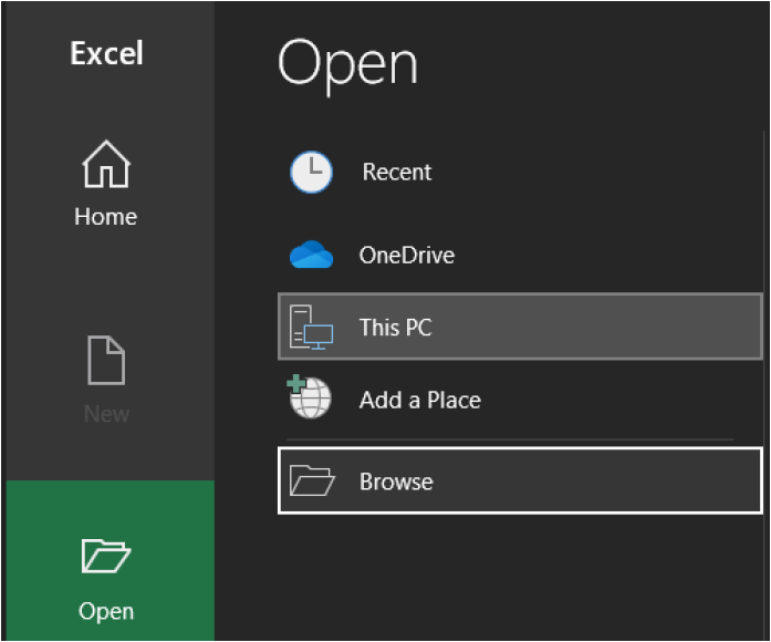
Step 3:

Browse to your desired Excel Worksheet saved with .xlsx extension

Step 4:

Double click on that sheet to work on it

---

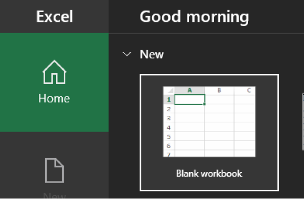
Creating new Excel Sheet

Step 1:

Select Blank Workbook under New Section

---

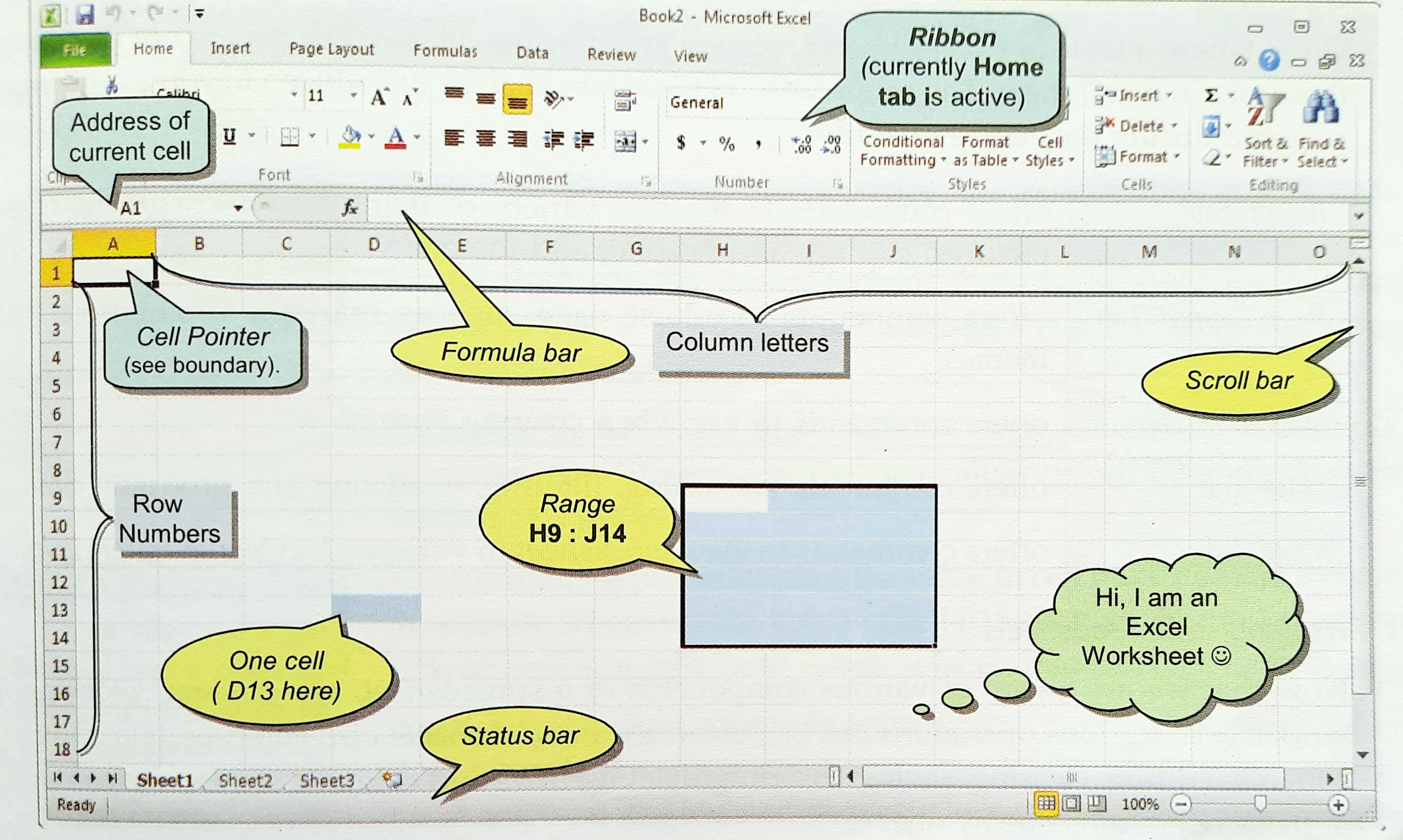
Introduction to Excel

Just below the title of your Worksheet, you can see different tabs grouped in a single line. This line is called ribbon which allows you to work smoothly and efficiently in any MS-Office tool you choose.

Let us take a quick look at Excel Ribbon

Home tab

By default, the Home tab is active. It incorporates all text and cell formatting features such as font and paragraph changes. It also includes basic spreadsheet formatting elements such as text wrap, merging cells, cell style, etc.

Insert tab

Offers commands to insert a variety of items into a document from pictures, shapes, links, tables and different charts

Page Layout tab

Offers commands to adjust page such as margins, orientation and themes

Formulas tab

Offers commands and operators to use when creating Formulas

Data tab

Offers commands for sorting, filtering, analyzing and grouping data

Review tab

Offers commands to review your work such as spelling and also helps you protect your sheet from malicious activities

View tab

Offers commands to view worksheet in variety of styles/layouts/views.

Quick Access toolbar

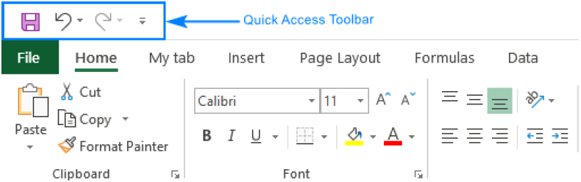
This toolbar helps to access save, undo and redo commands and we can also add commands later to it as per our repetition of using a basic command.

---

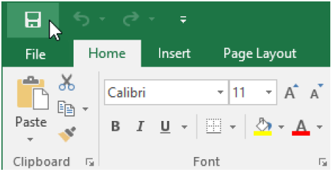
Saving a worksheet

Step 1:

Press Ctrl + S together on your keyboard or select save on the File tab or click the save icon on the Quick Access Toolbar

Step 2:

If you’re saving the workbook for the first time, then Save As dialog box pops up

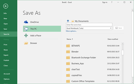
Step 3:

In the File name, type a name for the workbook.

Step 4:

Finally click Save to save the workbook completely.

However, if you are saving a workbook which was saved before, Excel will simply update the already saved Workbook.

Working on Excel

Now that we are aware of various components of a spreadsheet, we can startentering data, moving, copying, editing, clearing, saving, inserting/deleting rows and columns, etc on the spreadsheet.

Data Insertion

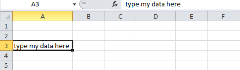
Any type of data – numeric, alphanumeric, text or formula can be entered in worksheets by typing. To enter data in a cell

Step 1:

Place the cell pointer over the desired cell

Step 2:

Type the data you wish to enter

---

Working With Formulas

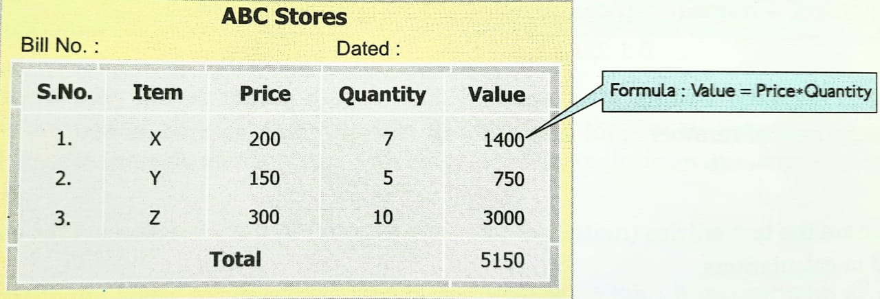
To obtain a similar bill in Excel

Step 1:

Enter the first two rows as in above figure, then move to next row.

Step 2:

Move to the next row and enter the headings S.No in 1st column, Item in 2nd Column, Price in 3rd Column, Quantity in 4th Column and Value in the 5th Column. Enter all the given entries except for the 5th column.

Step 3:

To obtain the values in 5th column, place the cell pointer in this column next to value 5 of Qty. Enter the formula =C6*D6 in MS-Excel and press Enter.

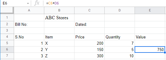
The moment you enter this formula, you see the calculated result get displayed on the worksheet.

Step 4:

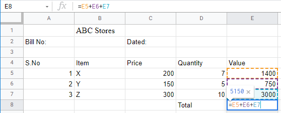
Similarly, get the values of other two rows and the total using * and + operation in Excel.

Hint for getting the total Value

Rearranging Worksheet

Editing Cell Contents

We can edit the cell contents in two ways

1) To edit a cell by overwriting, follow these steps

Step 1:

Select the cell you want to edit (You can select a cell by clicking over it or by using the arrow keys on keyboard)

Step 2:

Type in the new contents

Step 3:

Hit enter key on the keyboard.

2) To partially modify the cell contents without overwriting, follow these steps

Step 1:

Select the cell you want to edit

Step 2:

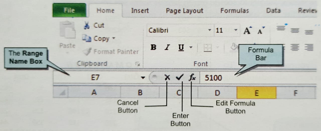
To edit its contents, either click the formula bar or press F2. Alternatively, you can double click the cell to be edited.

Step 3:

Edit the cell and press Enter key.

---

Selecting a range

A range is a continuous block of contiguous cells. Whenever an operation is performed on a range, it is performed on all the component cells of that range. We can select range either by using a keyboard or mouse.

In the above figure, the corner (active) cell is A4 and the selected range is A4:E8.

Selecting a range using Mouse

Step 1:

Point to a corner cell of the range to be selected. For example, if you want to select range A4:C7 then A4, A7, C4 and C7 are corner cells. You can point to any of these cells.

Step 2:

Now holding the left mouse button, drag the mouse pointer to the diagonally opposite corner of the cell. Example, if you had started earlier with A4, you need to drag the mouse pointer to C7.

Selecting a range using Keyboard

Step 1:

Point to a corner cell of the range to be selected.

Step 2:

Press Shift key. Holding Shift key, move to the diagonally opposite corner cell, using arrow keys.

Step 3:

Now release shift key.

Selecting multiple ranges

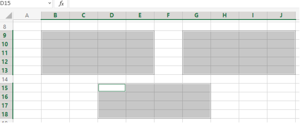
Note: Even on selecting multiple ranges, only one cell remains active, i.e, D15 here

In order to select multiple ranges together

Step 1:

Select first range

Step 2:

Hold down Ctrl key and select another range.

Step 3:

Repeat step 2 as long as you want to select multiple ranges together

Selecting complete row or column

To select the complete row or column, you just need to click row heading or column heading.

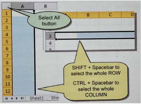
Selecting entire worksheet

To select the entire worksheet, press Ctrl + A or press Select All button

---

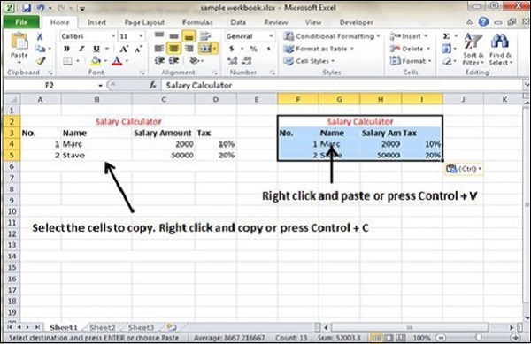
Copying & pasting a Range

To copy data from a source range to a destination range usecopy and Paste

Step 1:

Select the source range, i.e., the range to be copied

Step 2:

Press Ctrl + C keys together on your keyboard

Step 3:

Now select the target range, i.e., the range onto which the data are to be copied

Step 4:

Press Ctrl + V keys together on your keyboard

Another way to copy data is copying by dragging

Step 1:

Select the source range, i.e., the range to be copied

Step 2:

Position the mouse pointer on the border of selected range

Step 3:

Hold down Ctrl key. You’ll notice that the mouse pointer changes to an arrow with a plus sign. This indicates that copy operation has been initiated.

Step 4:

Drag the border to target location while holding the mouse’s left button

Step 5:

Release the mouse button

---

Erasing/Clearing ranges

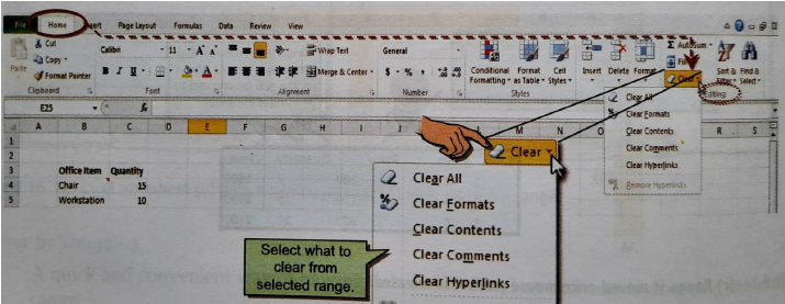
To clear cells completely or partially, you may follow these steps

Step 1:

Select the cells, rows or columns you want to clear

Step 2:

Click Home tab => Editing group => Clear dropdown menu and then click one of the four options of clear submenu: All, Formats, Contents,Comments or Hyperlinks.

All: MS-Excel will remove all cell contents and formatting including comments and hyperlinks from selected cells

Formats: Only cell formats are removed from selected cells

Contents: All data and formulas will be removed

Comments: All comments attached to selected cells will be removed

Hyperlinks: All hyperlinks ( links which redirect you to another file or another website) attached to selected cells will be removed

---

Naming a range

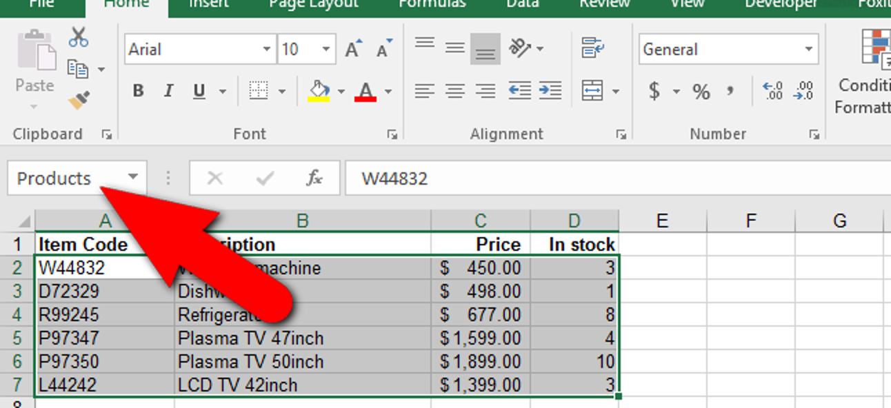
In the above fig, the entire range from A2:D7 is names as ‘Products’

Step 1:

Select the range to be named

Step 2:

Type the name, which is to be given to the selected range, in the Name box.

Some Useful Functions

While defining a function in Excel, there are two integral parts of it

1) Arguments: They are the values passed to the functions. They can be numbers, text, logical values such as TRUE or FALSE, ranges or cell references. They can also be constants, formulas or other functions.

2) Structure: The structure of a function begins with a function name, followed by open parenthesis then the arguments to be passed separated by commas, and a closing parenthesis as shown in figure below. If a function starts a formula, type an equal sign (=) before the function name.

Remember, string values get converted to numbers when passed as arguments.

Sum

This function adds all the numbers in a range of cells.

Its syntax is SUM (number1, number 2, …, number 30) where the total number of arguments can be at maximum 30.

Some important points to consider

a. Numbers, logical values and text representations of numbers that you type directly into the list of arguments are counted.

b. If an argument is an array, then only numbers in that array are counted.

c. Arguments that are text will be converted to numbers, if not possible to convert, then error will be raised.

Some important examples

a. =SUM (“2”,3) equals 5 because text values are translated into numbers

b. If cells A2:E2 contain 5, 15, 30, 40 and 50

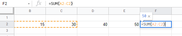
=SUM (A2:C2) equals 50 as it denotes A2 +B2+C2 = 5+15+30 = 50

Similarly,

=SUM (B2:E2,15) equals 150 as it denotes B2+C2+D2+E2+15 = 15+30+40+50+15 = 150

---

Average

This function returns the average (arithmetic mean) of the arguments.

Its syntax is AVERAGE (number 1, number 2, …, number 30)

The arguments must be either number or names, arrays or references that contain numbers. Cells with value zero are included.

Some examples

a. If range A1:A5 is named Scores and contain the numbers 10,7,9,27 and 2 =AVERAGE (A1:A5) equals 11

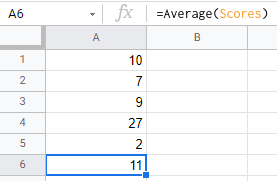
=AVERAGE(Scores) equals 11

b. If C1:C3 is named OtherScores and contain the numbers 4,18 and 7

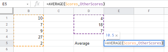
=AVERAGE (Scores, OtherScores) equals 10.5

---

Count

This function counts the number of cells that contain numbers and numbers within the list of arguments.

Its syntax is COUNT (value1, value2, …, upto value 30)

Arguments that are numbers, dates or text representation of numbers are counted. Arguments that are logical values or text which cannot be converted to numbers are ignored.

Let us better understand with an example

In the following example

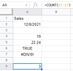
= COUNT (A1:A7) equals 3

= COUNT (A3:A5,2) also equals 3 as blank cells are ignored and it counts 19,22.24 and 2.

---

Max & Min

MAX

This function returns the largest value in a set of values.

Its syntax is MAX (number 1, …, number 30)

You can specify arguments that are numbers, empty cells, logical values or text representation of numbers. However, empty cells, text and logical values get ignored.

If logical values and text must not be ignored, use MAXA () instead of MAX ().

Example:

If A1:A5 contains the numbers 7,10,9,27 and 2 then:

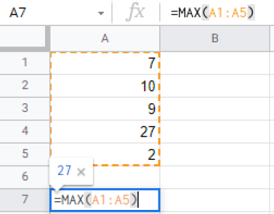
=MAX (A1:A5) gives 27.

= MAX (A1:A5,30) gives 30.

MIN

This function returns the smallest value in a set of values.

Its syntax is MIN (number 1,number 2, …, number 30)

You can specify arguments that are numbers, empty cells, logical values or text representation of numbers. However, empty cells, text and logical values get ignored.

If logical values and text must not be ignored, use MINA () instead of MIN ().

Example:

If A1:A5 contains the numbers 7,10,9,27 and 2, then

= MIN (A1:A5) gives 2.

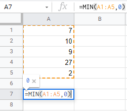
= MIN (A1:A5,0) gives 0.

Formatting Data

The general arrangement of data is known as formatting. It is the formatting that makes your worksheet neat and presentable. There are several aspects of formatting like text formatting, number formatting, date formatting and formatting the entire cell. Let us look at each one of these one by one

Formatting text

To change the font

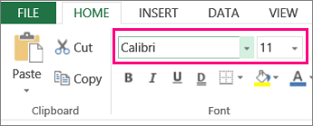
Step 1:

Select the cells to be formatted

Step 2:

Click the Home tab => Font group => Font box’s drop-down arrow. The font drop-down menu appears.

Step 3:

Move your mouse over the various fonts. A live preview of the font will appear in the worksheet.

Step 4:

From the drop-down list of fonts, select the font you want to use.

To change the font size

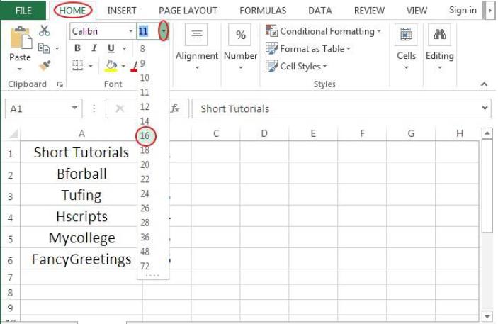
Step 1:

Select the cells to be formatted

Step 2:

Click the Home tab => Font group => Font-size box’s drop-down arrow. The font-size drop-down menu appears.

Step 3:

Move your mouse over the various font sizes. A live preview of the font-size will appear in the worksheet.

Step 4:

Select the font size you want to use.

To Bold, Italic or Underline text

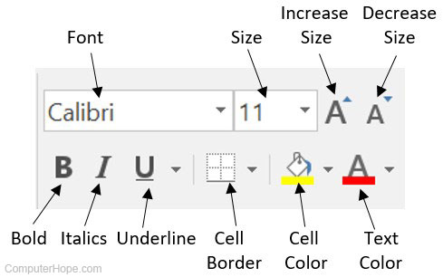
Step 1:

Select the cells to be formatted

Step 2:

Click the Bold (B), Italic (I), Underline (U) commands on the Home tab => Font group

To add a border

Step 1:

Select the cells to be formatted

Step 2:

Click the Home tab => Font group => the drop-down arrow next to Borders command. The border drop-down menu appears.

Step 3:

Select the border style you want to use.

To change the font/text colour

Step 1:

Select the cells to be formatted.

Step 2:

Click the Home tab => Font group => Font colour’s drop-down arrow. The colour menu appears.

Step 3:

Move your mouse over the various font colours. A live preview of the colour will appear in the worksheet

Step 4:

Select the font colour you want to use.

To change horizontal text alignment

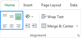
Step 1:

Select the cells to be formatted

Step 2:

Select one of the three horizontal alignments commands on the Home tab => Alignment group.

1. Align text left: Aligns text to the left of the cell.
2. Center: Aligns text to the center of the cell.
3. Align text right: Aligns text to the right of the cell.

To change vertical text alignment

Step 1:

Select the cells to be formatted

Step 2:

Select one of the three vertical alignments commands on the Home tab => Alignment group.

1. Top Align: Aligns text to the top of the cell.
2. Middle Align: Aligns text to the middle of the cell.
3. Bottom Align: Aligns text to the bottom of the cell.

---

Formatting Numbers and Dates

This formatting is used to format numbers with decimal places, currency symbol (₹), percent symbol (%), etc.

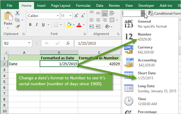
Step 1:

Select the cells to be formatted.

Step 2:

Click Home tab => Number group => drop-down arrow next to the Number Format command.

Step 3:

From the format drop-down menu that appears, select the number format you want.

---

Formatting Cells Dailog

This formatting is used to do all types of formatting.

Step 1:

Select the cells to be formatted.

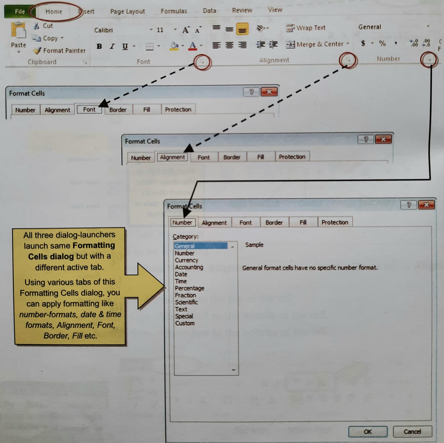
Step 2:

Click the dialog launcher from Home’s tab Font group or Alignment group or Number group as shown in above figure.

Step 3:

Every time the same Formatting Cells dialog will be launched with a different tab.

Creating a chart

There are two ways in which we can create a chart in MS-Excel. These are

Using F11 function key

Step 1:

Select the cell range from the worksheet.

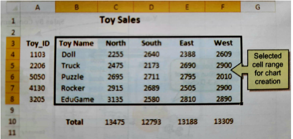
Step 2:

Press the F11 key. It will create a column bar chart with selected data and add a separate Chart sheet to your worksheet.

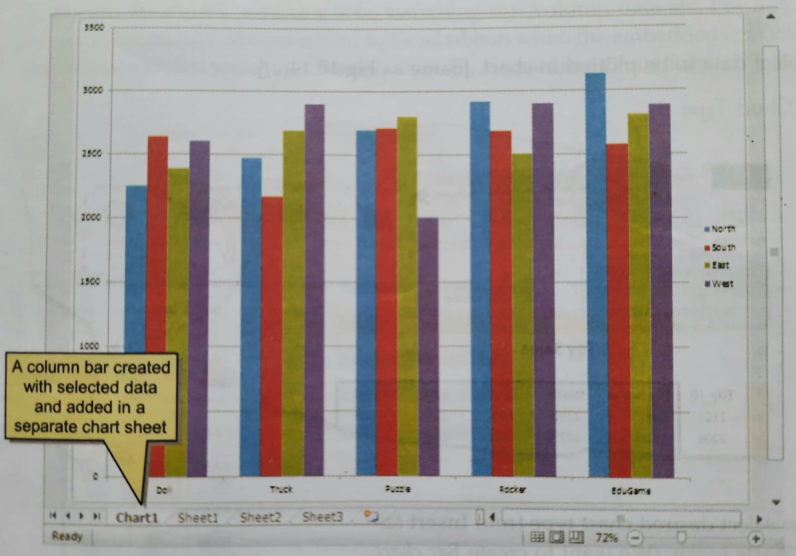
Step 3:

You can click on the data sheet’s tab to get back your data.

Creating chart with Insert Chart type method

Step 1:

Select the cell range from the worksheet. You must select all the cells containing the data you want in your chart. You should also include the data labels. (Make sure that the data selected forms a rectangular range)

Step 2:

Click the Insert tab

Step 3:

Select the Chart Type from Charts group

Step 4:

Format the chart as preferred

Format your Chart

Now that you have a primitive chart visible to you, you can format the chart by adding Chart title, axes titles, adjusting size, switching row/column data etc. For this you will use the contextual tabs: Design, Layout, Format and Chart tools

Add chart title

Step 1:

Select the chart

Step 2:

From the contextual tabs, click Layout tab => Labels group => Chart title => Centered Overlay Title/ Above Chart

Step 3:

It will add a Chart title to the chart. Click on the Chart title placeholder and type your own text.

Add Axes title

Step 1:

Select the chart

Step 2:

From the contextual tabs, click Layout tab => Labels group => Axis Titles => Primary Horizontal Axis title / Primary Vertical Axis title.

Step 3:

It will add axes titles to the chart as per your selection. Click on the placeholder and type your own text as you did for the chart title.

Printing Worksheets/Charts

To print an entire worksheet, follow these steps

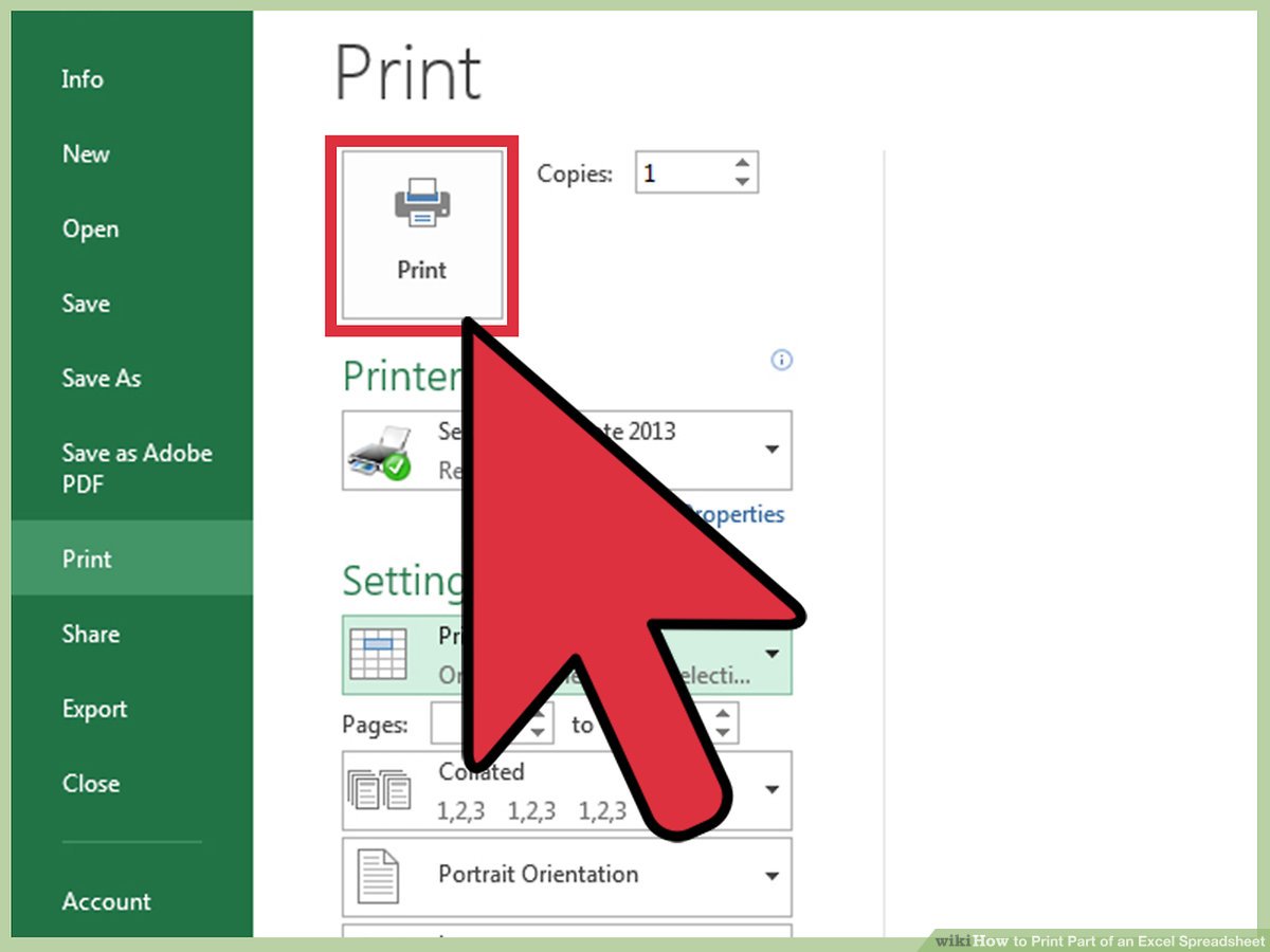
Step 1:

On the File menu, click Print.

Step 2:

A print section will appear

Step 3:

In this section, under settings select the option you want.

1. Choose Print Selection only if you want to print a selected range which must have already been selected by you.
2. Choose Print active sheet(s) option, if you want to print all the selected sheets.
3. Choose Print Entire Workbook option, if you want to print entire workbook.
4. If you have selected a chart before you invoke Print command, Print what offers an option Selected chart.

Step 4:

Enter the desired number of printed copies in the box named Copies.

Step 5:

Click OK to confirm.

Quiz

You've learnt a lot of things.

Are you ready to take a small quiz?

Try it NOW !!!

---